GRN Inference: P21 Mouse Brain

STARNet workflows have two main parts: model training, followed by gene regulatory network (GRN) module inference. The inferred GRNs can then be reused for downstream analyses such as spatial trajectory inference, GWAS interpretation, and drug response analysis.

This tutorial uses paired spatial RNA and ATAC data from P21 mouse brain. It walks through STARNet training, GRN inference, module scoring, visualization, and downstream analyses. The trained spot and gene embeddings are reused as inputs for GRN inference.

import warnings
import os
warnings.filterwarnings("ignore")
os.environ["PYTHONWARNINGS"] = "ignore::FutureWarning"

import scanpy as sc
import anndata as ad
import STARNet as ST
import pandas as pd
import pickle

Stage 1: Model Training and GRN Inference

Read data

This tutorial uses the P21 mouse brain dataset. Download the tutorial data from Links to Data Folder, then place the Drive folder next to this notebook so paths such as Drive/Datasets/P21_Mouse/... resolve correctly. You can download only the files used here or the full data folder.

adata_rna = sc.read_h5ad("Drive/Datasets/P21_Mouse/Raw_Data/adata_rna.h5ad")
adata_atac = sc.read_h5ad("Drive/Datasets/P21_Mouse/Raw_Data/adata_atac.h5ad")

Here, we create a ST.model.STARNet object from the paired RNA and ATAC AnnData objects. If a GPU is available, set device='cuda:N' to choose the GPU used for training.

starnet_obj = ST.model.STARNet(adata_rna, adata_atac, device='cuda:1')

Next, preprocess() prepares the paired multi-omics data for model training. This step performs quality control, selects highly variable genes and peaks, normalizes the data, and constructs the required scRNA, scATAC, cell-neighbor, and peak-to-gene graphs.

starnet_obj.preprocess()

==================================================
Step 1: Data Alignment and Initialization
📄 Data Alignment Results:
   ✓ adata_rna: Dataset shape: 2373 spots × 19859 genes
   ✓ adata_atac: Dataset shape: 2373 spots × 135463 peaks
Converting adata_rna.X to csr_matrix format.
✅ Conversion complete.

==================================================
Step 2: Processing RNA Data
Filtering genes: min_cells=15
Running RNA Leiden clustering (res=0.2)...

==================================================
Step 3: Processing ATAC Data
Selecting top 40000 ATAC peak features.
Running ATAC Leiden clustering (res=0.2)...
Final RNA shape: (2373, 12667)
Final ATAC shape: (2373, 40000)

==================================================
Step 4: Building Heterogeneous HyperGraph
🧬 RNA graph nodes prepared: 12667 genes
🧩 ATAC graph nodes prepared: 40000 peaks
Building Dual-Modality Spot-Spot matrices...
Using 'leiden' clusters from obs.
Constructed dual-modality matrix for K=3.
Constructed dual-modality matrix for K=4.
Constructed dual-modality matrix for K=8.
 ✅ Graph data moved to device: cuda:1

We then train STARNet for 600 epochs, which is the recommended setting for these tutorial datasets. Training stores the spot/cell embedding in adata_rna.obs and the gene embedding in adata_rna.uns for later GRN inference.

starnet_obj.train(epochs=600, eval_every=600)

==================================================
🔍 Step 1: STARNet Model Initialization and Configuration
📄 Model Parameters:
   ✓ Hidden Dim: 128
   ✓ Output Dim: 128
   ✓ Device: cuda:1
   ✓ SSL Num Neg: 10240
Lightning model built with ComplexConv_v4 architecture.

==================================================
🔍 Step 2: Starting STARNet Training Loop
📄 Training Configuration:
   ✓ Max Epochs           : 600
   ✓ Device               : cuda:1
   ✓ Evaluation Every     : 600 epochs
   ✓ Checkpointing        : True
   ✓ TensorBoard Log Dir  : ./lightning_logs/STARNet/version_5
==================================================
📊 Epoch Summary: epoch=1/600, best_total_loss=6.5488
📊 Epoch Summary: epoch=600/600, best_total_loss=0.4179
Evaluating clustering using representation 'cell_embedding'...
==================================================
📊 Training Summary:
   ✓ Completed Epochs     : 600
   ✓ Best Total Loss      : 0.4179
 ✅ Epoch-level training visualization finished.
==================================================
✅ Training finished!
   ✓ TensorBoard logs saved to: ./lightning_logs/STARNet/version_5
   ✓ Checkpoints saved to: ./lightning_logs/checkpoints

The trained RNA AnnData object is shown below and saved for reuse in the GRN inference steps.

print(f'RNA data after training: {starnet_obj.adata_rna}')
starnet_obj.adata_rna.write_h5ad("Drive/Datasets/P21_Mouse/Process_Data/adata_rna_trained.h5ad", compression='gzip')

RNA data after training: AnnData object with n_obs × n_vars = 2373 × 12667
    obs: 'n_genes_by_counts', 'log1p_n_genes_by_counts', 'total_counts', 'log1p_total_counts', 'pct_counts_in_top_50_genes', 'pct_counts_in_top_100_genes', 'pct_counts_in_top_200_genes', 'pct_counts_in_top_500_genes', 'total_counts_mt', 'log1p_total_counts_mt', 'pct_counts_mt', 'total_counts_ribo', 'log1p_total_counts_ribo', 'pct_counts_ribo', 'total_counts_hb', 'log1p_total_counts_hb', 'pct_counts_hb', 'leiden', 'pre_clusters'
    var: 'mt', 'ribo', 'hb', 'n_cells_by_counts', 'mean_counts', 'log1p_mean_counts', 'pct_dropout_by_counts', 'total_counts', 'log1p_total_counts', 'n_cells'
    uns: 'log1p', 'pca', 'neighbors', 'leiden', 'umap', 'gene_embedding', 'pre_clusters_colors', 'leiden_colors'
    obsm: 'X_spatial', 'X_pca', 'cell_embedding', 'X_umap'
    varm: 'PCs'
    obsp: 'distances', 'connectivities'

Load multi-omics data

For GRN inference, you can either continue with the AnnData object trained above or load the pre-trained dataset provided with the tutorial files.

# Load data from the trained model or from a saved state

# optional
# adata_rna = starnet_obj.adata_rna
# adata_atac = starnet_obj.adata_atac

adata_rna = sc.read_h5ad('Drive/Datasets/P21_Mouse/Process_Data/adata_rna_trained.h5ad')
adata_rna_raw = sc.read_h5ad("Drive/Datasets/P21_Mouse/Raw_Data/adata_rna.h5ad")
adata_atac = sc.read_h5ad("Drive/Datasets/P21_Mouse/Raw_Data/adata_atac.h5ad")

Before GRN inference, we add the raw RNA counts to the count layer because the downstream GRN calculations use raw count values.

# Gene embedding
adata_rna.uns['gene_embedding'] = ad.AnnData(
    adata_rna.uns['gene_embedding'],
    obs=pd.DataFrame(index=adata_rna.var_names)
)

# Clean cell names
for x in [adata_rna, adata_rna_raw, adata_atac]:
    x.obs_names = [i.split('-')[0] for i in x.obs_names]

# Add raw counts
adata_rna.layers['counts'] = adata_rna_raw[adata_rna.obs_names, adata_rna.var_names].X
adata_atac.layers['counts'] = adata_atac.X.copy()

print(f'RNA data info:\n{adata_rna}')
print(f'ATAC data info:\n{adata_atac}')

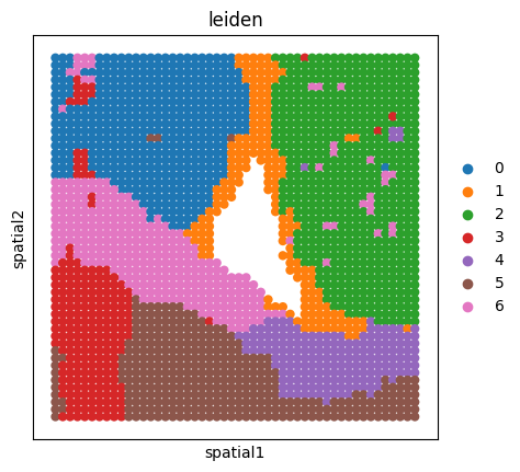
sc.pl.spatial(adata_rna, color='leiden', spot_size=1.25)

RNA data info:
AnnData object with n_obs × n_vars = 2373 × 12667
    obs: 'n_genes_by_counts', 'log1p_n_genes_by_counts', 'total_counts', 'log1p_total_counts', 'pct_counts_in_top_50_genes', 'pct_counts_in_top_100_genes', 'pct_counts_in_top_200_genes', 'pct_counts_in_top_500_genes', 'total_counts_mt', 'log1p_total_counts_mt', 'pct_counts_mt', 'total_counts_ribo', 'log1p_total_counts_ribo', 'pct_counts_ribo', 'total_counts_hb', 'log1p_total_counts_hb', 'pct_counts_hb', 'leiden', 'pre_clusters'
    var: 'mt', 'ribo', 'hb', 'n_cells_by_counts', 'mean_counts', 'log1p_mean_counts', 'pct_dropout_by_counts', 'total_counts', 'log1p_total_counts', 'n_cells'
    uns: 'gene_embedding', 'leiden', 'leiden_colors', 'log1p', 'neighbors', 'pca', 'pre_clusters_colors', 'umap'
    obsm: 'X_pca', 'X_spatial', 'X_umap', 'cell_embedding'
    varm: 'PCs'
    layers: 'counts'
    obsp: 'connectivities', 'distances'
ATAC data info:
AnnData object with n_obs × n_vars = 2373 × 135463
    obs: 'n_fragment', 'frac_dup', 'frac_mito', 'Sample'
    obsm: 'X_spatial'
    layers: 'counts'

Load genomic reference files and infer GRNs

With the multi-omics data prepared, we load the genomic reference folder and infer GRNs. use_rep selects the embedding used to group similar spots/cells. pvalue_regulatory=0.2 controls the p-value threshold for candidate cis-regulatory links, and moranI_threshold=0.01 keeps transcription factors with Moran’s I scores above the threshold as spatially variable regulators.

genomic_data_pathway = 'Drive/Datasets/Reference/mouse_vM25'
adata_rna = ST.grn.infer_grn_from_multiomics(adata_rna,
                                             adata_atac,
                                             genomic_data_pathway,
                                             use_rep='cell_embedding',
                                             pvalue_regulatory=0.2,
                                             moranI_threshold=0.01,
                                             n_jobs=5)

==================================================
🧬 Starting Spatially Specific GRN Inference Pipeline in STARNet
==================================================

==================================================
🔍 Step 1: Identifying Genomic Reference Files
📄 Target Directory: Drive/Datasets/Reference/mouse_vM25
✅ Genomic files identified and validated.
📄 File Discovery Results:
   ✓ Motif File        : cisBP_mouse.meme
   ✓ Genome Fasta      : gencode_vM25_GRCm38.fa
   ✓ Annotation (GFF)  : gencode_vM25_GRCm38.gff3
   ✓ Annotation (GTF)  : gencode_vM25.chr_patch_hapl_scaff.annotation.gtf
 ✅ Reference genome and annotation paths successfully loaded.

==================================================
🔍 Step 2: Peak GC Content Analysis
 ⚙️ Calculating GC proportion for peaks of spatial ATAC-seq data...

==================================================
🔍 Step 3: Spatially Specific Transcription Factor Identification
 ⚙️ Identifying TFs with significant spatial patterns (Moran's I > 0.01)...
   ✓ Identify spatially-variable expressed TFs: 148

==================================================
🔍 Step 4: Genomic Data Alignment and Formatting
✅ Genomic data preparation successful.
📄 Processed Stats:
   ✓ RNA spots/genes  : 2373 × 11489
   ✓ ATAC spots/peaks : 2373 × 135449
   ✓ Aligned Genes    : 11489

==================================================
🔍 Step 5: Primary GRN Construction (Embedding Similarity)
 ⚙️ Calculating target genes using vectorized cosine similarity...
   ✓ Total TFs processed : 148
   ✓ Total Interactions  : 74000
 ✅ Primary GRN construction complete.

==================================================
🔍 Step 6: Metacell Generation
⚠️ CuPy is not installed. Switching to CPU mode. To use GPU acceleration, please install CuPy (https://github.com/cupy/cupy).
 ⚙️ Calculate the metacells for spatial RNA-seq and spatial ATAC-seq data by using SEACells...
 ⚙️ Building kernel on cell_embedding...
   ✓ Generated 31 metacells.

==================================================
🔍 Step 7: GRN Filtering (Stage1)
 ⚙️  Calculating correlations for 74000 interactions...
 📄 Processed Stats:
   ✓ Threshold                   : >0.2
   ✓ Initial TF-target Pairs     : 74000
   ✓ Passed TF-target Pairs    : 28082
   ✓ Removal TF-target Rate      : 62.05%
✅ Correlation filtering complete.
 ⚙️ Mapping peaks to genes (100kb around gene body)...
 📄 Processed Stats:
   ✓ Expand Range    : +/- 100,000 bp
   ✓ Initial Pairs   : 28082
   ✓ Validated Pairs : 27966
   ✓ Removal Rate    : 0.41%
✅ Peak filtering complete.

==================================================
 ⚙️ Step 8: GRN Filtering using Peak-to-Gene Links (Stage2)
Loading transcripts per gene...
Preparing matrices for gene-peak associations
Computing peak-gene correlations
 📄 Processed Stats:
    ✓ Initial Peak-to-Gene Links     : 198,192
    ✓ Significant Peak-to-Gene Links : 51,644
    ✓ Removal Rate                  : 73.94%
✅ Peak-to-Gene filtering complete.

==================================================
🔍 Step 9: Parallel Motif Scanning
 ⚙️ Identify the motif corresponding to specific transcription factors...

==================================================
📊 Finally Spaitally Specific GRN Inference Results:
==================================================
 📊 Final Network Summary:
   ✓ Total Target Genes          : 5,292
   ✓ Total Regulatory Peaks      : 28,147
   ✓ Total TF-Target Interactions: 13,991
 ✅ Network added to .uns['grn_df'] and regulatory peaks to .uns['regulatory_peaks']
==================================================

Next, we extract peak-to-gene associations from the GTF gene annotation file in the reference folder. These links connect candidate cis-regulatory elements with nearby genes, allowing STARNet to associate TF binding with spatially specific target gene expression.

gtf_pathway = 'Drive/Datasets/Reference/mouse_vM25/gencode_vM25.chr_patch_hapl_scaff.annotation.gtf.gz'
peak2gene = ST.pp.extract_peak_gene_associations(adata_rna,gtf_file=gtf_pathway)
peak2gene.to_csv('Drive/Datasets/P21_Mouse/Process_Data/peak2gene.links', sep="\t", index=False)

==================================================
🔗 Extracting Peak-Gene Associations for Visualization
==================================================
 ⚙️ Loading GTF and aligning gene coordinates...
 ⚙️ Aggregating Peak-to-Gene links from .uns['Peak2Gene']...
 ⚙️ Parsing genomic coordinates...
 ⚙️ Calculating scores and formatting...
==================================================
 📊 Association Extraction Summary:
   ✓ Total Raw Links      : 51,644
   ✓ Self-loops Removed   : 9
   ✓ Final Associations   : 51,635
 ✅ Formatting complete.
==================================================

After inferring GRNs and peak-to-gene links, we score each GRN and TF module to quantify how strongly each transcription factor regulates its target genes. These scores support GRN visualization and can also be used as edge weights for downstream cell reprogramming analysis with PriciCE.

# Perform permutation test on all gene regulatory networks
adata_rna = ST.pp.score_all_grn(adata_rna,n_jobs=5)

# Calculate the TF module using various clustering methods and perform cauchy combination tests
adata_rna = ST.pp.score_TF_module(adata_rna,
                                  clustering_method='leiden',
                                  resolution = 2,
                                  groupby='leiden',n_jobs=5)

==================================================
🧬 Calculating GRN Significance via Permutation Test
==================================================
 ⚙️ Starting parallel scoring for 148 GRNs...
==================================================
 ✅ Scoring complete! Results stored in:
  Full GRN score AnnData: added to .uns['grn']['adata_nlog10_pval']
==================================================

==================================================
🧬 TF Module Analysis: Clustering & Significance
==================================================
 ⚙️ Preprocessing and running leiden clustering...
 ✅ Leiden clustering finished: 10 clusters found.
 ⚙️ Scoring 10 TF modules in parallel...
--------------------------------------------------
 ✨ All tasks completed successfully!
  1. TF Gene Lists:       added to .uns['TF_module']['TF_list']
  2. Target Gene Lists:   added to .uns['TF_module']['target_gene_list']
  3. Score AnnData:       added to .uns['TF_module']['nlog10_pval_ad']
  4. Cauchy Results:      added to .uns['TF_module']['cauchy_combination_test']
==================================================

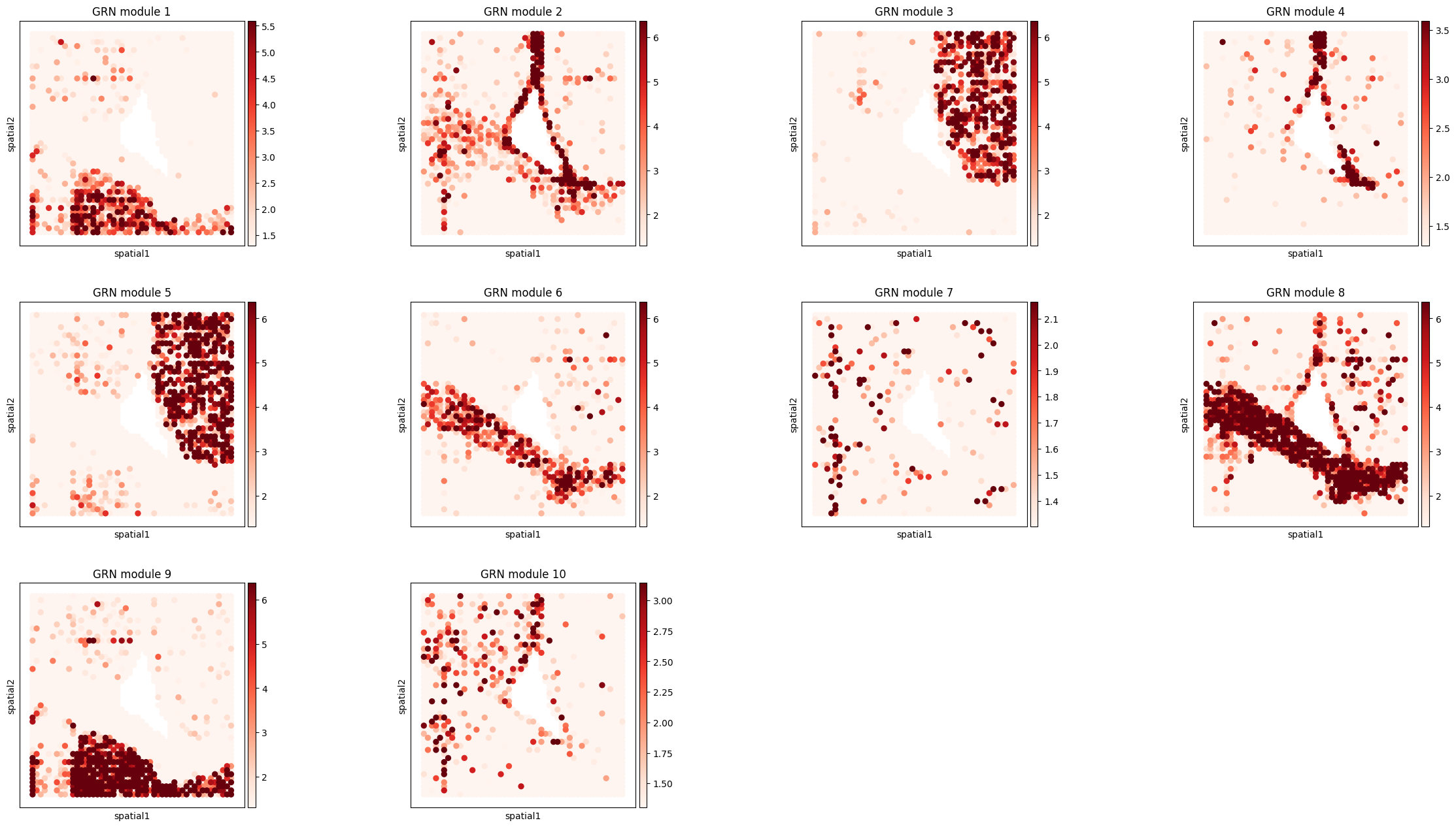
Visualize GRN modules

The following cell plots GRN module activity in spatial coordinates. The module patterns should align with known anatomical regions in the P21 mouse brain.

import matplotlib.pyplot as plt
import scanpy as sc
import numpy as np
import anndata as ad

mod_ad = ad.AnnData(adata_rna.uns['TF_module']['nlog10_pval_df'][[str(i) for i in range(10)]])
mod_ad.obsm['spatial'] = adata_rna[mod_ad.obs_names].obsm['spatial']
mod_ad.var_names = [f'GRN module {int(i) + 1}' for i in mod_ad.var_names]

sc.pl.spatial(
    mod_ad,
    color=mod_ad.var_names,
    cmap='Reds',
    spot_size=1.5,
    vmin=-np.log10(0.05),
    vmax='p98',
    ncols=4,
)

adata_rna.write_h5ad("Drive/Datasets/P21_Mouse/Process_Data/adata_rna_GRN.h5ad",compression="gzip")

Stage 2: Downstream Analysis

This stage demonstrates how to reuse the inferred GRNs and TF modules for downstream analyses, including spatial domain visualization, top-module ranking, TF-TF interaction networks, GO enrichment, genome-track visualization, and peak-to-gene link inspection.

import os
os.environ["CUDA_VISIBLE_DEVICES"] = "0"  # Set to the GPU you want to use, or set to "" for CPU only

import warnings
warnings.simplefilter("ignore", FutureWarning)

import matplotlib.pyplot as plt
import STARNet as ST
# import omicverse as ov
import scanpy as sc
import numpy as np
import pandas as pd

# fb=ov.pl.ForbiddenCity()
# ov.plot_set()
sc.settings.set_figure_params(vector_friendly=True)
plt.rcParams['pdf.fonttype'] = 42
plt.rcParams['ps.fonttype'] = 42

def rotate_points_90_degrees_counterclockwise(points):
    rotated_points = np.array([-points[:, 1], points[:, 0]]).T
    return rotated_points

We first reload the RNA AnnData object, GRN results, and TF modules generated in Stage 1.

adata_rna = sc.read_h5ad('Drive/Datasets/P21_Mouse/Process_Data/adata_rna_GRN.h5ad')
print(f'RNA-seq Info: {adata_rna}')

RNA-seq Info: AnnData object with n_obs × n_vars = 2373 × 12667
    obs: 'n_genes_by_counts', 'log1p_n_genes_by_counts', 'total_counts', 'log1p_total_counts', 'pct_counts_in_top_50_genes', 'pct_counts_in_top_100_genes', 'pct_counts_in_top_200_genes', 'pct_counts_in_top_500_genes', 'total_counts_mt', 'log1p_total_counts_mt', 'pct_counts_mt', 'total_counts_ribo', 'log1p_total_counts_ribo', 'pct_counts_ribo', 'total_counts_hb', 'log1p_total_counts_hb', 'pct_counts_hb', 'leiden', 'pre_clusters'
    var: 'mt', 'ribo', 'hb', 'n_cells_by_counts', 'mean_counts', 'log1p_mean_counts', 'pct_dropout_by_counts', 'total_counts', 'log1p_total_counts', 'n_cells', 'chrom', 'chromStart', 'chromEnd', 'strand'
    uns: 'Origin_Peak2Gene', 'Peak2Gene', 'TF_module', 'gene_embedding', 'grn', 'grn_df', 'leiden', 'leiden_colors', 'log1p', 'moranI', 'neighbors', 'pca', 'pre_clusters_colors', 'regulatory_peaks', 'spatial_neighbors', 'umap'
    obsm: 'X_pca', 'X_spatial', 'X_umap', 'cell_embedding', 'spatial'
    varm: 'PCs'
    layers: 'counts'
    obsp: 'connectivities', 'distances'

# GRN inference results 
adata_rna.uns['grn_df']

	TF	target gene	Cosine similarity	Pearson correlation
0	Dlx5	Mfap2	0.206482	0.370206
1	Dlx5	Ubfd1	0.193181	0.206384
2	Dlx5	Srgap2	0.310410	0.280055
3	Dlx5	Wscd2	0.196971	0.415842
4	Dlx5	Racgap1	0.193278	0.250182
...	...	...	...	...
13986	Nfatc3	Gm15445	0.246117	0.275197
13987	Nfatc3	Eps8l1	0.284011	0.369659
13988	Nfatc3	Timp4	0.255100	0.204443
13989	Nfatc3	Shc1	0.317650	0.293435
13990	Nfatc3	Nfic	0.295742	0.431543

13991 rows × 4 columns

Spatial domain visualization

Here, we annotate spatial domains in the mouse brain and visualize their locations across the tissue section.

Note

Because Leiden clustering can produce different cluster IDs across environments, the cluster-to-domain annotation used below may not match your reproduced result exactly. If your clusters differ from the tutorial output, adjust the cluster-to-annotation mapping according to the spatial domains shown in the reference annotation result before running downstream analyses.

adata_rna.obsm['spatial'] = rotate_points_90_degrees_counterclockwise(adata_rna.obsm['spatial'])
adata_rna.obsm['spatial'] = rotate_points_90_degrees_counterclockwise(adata_rna.obsm['spatial'])

fig, ax = plt.subplots(figsize=(3, 3))
ax = sc.pl.spatial(adata_rna,
              color=['leiden'], colorbar_loc=None,
              ncols=3, spot_size=1.25,legend_fontsize=12,
              ax=ax,show=False
             ) 
ax[0].set_title('STARNet', fontweight='bold',fontsize=13)
ax[0].set_xlabel('', fontsize=12)
ax[0].set_ylabel('', fontsize=12)

Text(0, 0.5, '')

# Short labels for analysis
ann = {
    '0': 'LS',
    '1': 'VL',
    '2': 'CP',
    '3': 'ACA',
    '4': 'CCB',
    '5': 'CTX',
    '6': 'CCB',
}

order = ['ACA', 'CCB', 'CP', 'CTX', 'LS', 'VL']

adata_rna.obs['spatial domain'] = (
    adata_rna.obs['leiden']
    .astype(str)
    .map(ann)
    .astype('category')
    .cat.reorder_categories(order)
)

adata_rna.uns['spatial domain_colors'] = [
    '#B793BD', '#FB7E00', '#C24A7A', '#FF9A9B', '#c9dcc4', '#E31A1C'
]

sc.pl.spatial(
    adata_rna,
    color='spatial domain',
    spot_size=1.25,
    title='Spatial domain',
    frameon=False,
)

Top GRN visualization

The top GRNs are visualized with a horizontal bar plot. For each spatial domain, module-level evidence is aggregated with the Cauchy combination test and displayed as -log10(P) values.

results_df = ST.pp.cal_cauchy_combination_test(adata_rna,annotation_col='spatial domain')
results_df = results_df.apply(pd.to_numeric, errors='coerce')
results_df = results_df.apply(lambda x: x.fillna(0))
results_df

	ACA	CCB	CP	CTX	LS	VL
E2f7	0.388867	0.435783	0.042777	0.002333	0.037748	1.683088
Ctcf	0.003706	0.000031	4.828212	0.000027	0.006352	0.010279
Pbx3	0.006224	0.000067	4.122084	0.000042	0.052679	1.897948
Foxj1	0.394115	0.197314	0.005419	0.000057	0.032130	5.403474
Mafb	0.170645	0.284498	0.086597	0.009405	0.072582	0.135984
...	...	...	...	...	...	...
Nr6a1	0.131383	0.000140	0.028599	2.133897	1.614014	0.000218
Kdm2b	0.266040	0.028990	0.032154	0.239703	0.037996	0.775982
Homez	0.294983	0.675122	0.082077	0.019081	0.091340	0.111189
Tcf7l2	0.014104	5.545139	0.000012	0.000013	0.000047	4.780001
Egr2	0.007078	0.000035	4.415235	0.004508	0.075131	0.000025

148 rows × 6 columns

import seaborn as sns
import matplotlib.pyplot as plt


marker_genes = {
    'CCB': ['Tcf4', 'Sox8', 'Sox10', 'Elf1', 'Sox2', 'Olig1', 'Olig2'],
    'CP':  ['Rreb1', 'Meis2', 'Foxp1', 'Foxp2', 'Rarb', 'Pou3f1', 'Cux1', 'Six3', 'Myt1l'],
    'CTX': ['Mef2c', 'Tbr1', 'Nr4a3', 'Sox5', 'Neurod2'],
    'VL':  ['Sox4', 'Otx2', 'Pou2f1', 'Dlx1', 'Sox9', 'Pou3f2', 'Arx'],
}

regions = ['ACA', 'CCB', 'CP', 'CTX', 'LS', 'VL']
genes = [g for gs in marker_genes.values() for g in gs]

plot_df = results_df.loc[genes, regions].T
plot_df.columns = [f'{g}(+)' for g in plot_df.columns]

g = sns.clustermap(
    plot_df,
    cmap='RdYlBu_r',
    vmin=-2,
    vmax=5,
    row_cluster=False,
    col_cluster=False,
    linewidths=0,
    linecolor=None,
    figsize=(13, 4),
)
g.ax_heatmap.grid(False)

plt.show()

from matplotlib.colors import ListedColormap

# Compute TF enrichment across spatial domains
result_df = ST.pp.cal_cauchy_combination_test(adata_rna, 'spatial domain')
result_df.index = result_df.index + '(+)'

# Select top TFs in CP from module 2
region = 'CP'
tf_list = [f'{tf}(+)' for tf in adata_rna.uns['TF_module']['TF_list']['2']]
plot_df = result_df.loc[tf_list].sort_values(region, ascending=False).head(12)

# Plot
ST.pl.horizontal_bar_chart(
    plot_df,
    values=region,
    figsize=(1.2, 3.4),
    xlabel='-log$_{10}$ $\it{P}$',
    ylabel='',
    vmin=0,
    vmax=result_df.max().max(),
    cmap=ListedColormap(['#C25759']),
)

==================================================
📊 Horizontal Bar Chart Generation
⚙️ Plot Configuration:
   ✓ Figure size: (1.2, 3.4)
   ✓ Colormap: from_list
   ✓ Font size: 14
   ✓ X-label: '-log$_{10}$ $\it{P}$'
✅ Horizontal bar chart generated successfully!
   ✓ Number of bars: 12
   ✓ Y-axis categories: 12
==================================================

<Axes: xlabel='-log$_{10}$ $\\it{P}$'>

gene = "Foxp1"

fig, ax = plt.subplots(figsize=(3, 3))

sc.pl.spatial(
    adata_rna,
    color=gene,
    vmin="p60",
    vmax=3.5,
    spot_size=1.25,
    legend_loc=None,
    ax=ax,
    show=False,
)

xmin, xmax = ax.get_xlim()
ymin, ymax = ax.get_ylim()
ax.set_xlim(xmin + 0.04 * (xmax - xmin), xmax - 0.04 * (xmax - xmin))
ax.set_ylim(ymin + 0.04 * (ymax - ymin), ymax - 0.04 * (ymax - ymin))

ax.set_title(gene, fontweight="bold", fontsize=15)
ax.set_xlabel("")
ax.set_ylabel("")

Text(0, 0.5, '')

TF-TF interactions

The following code visualizes TF-TF interaction networks. Directed edges indicate inferred regulatory relationships between transcription factors.

result_df = ST.pp.cal_cauchy_combination_test(adata_rna,'spatial domain')

tf_list = adata_rna.uns['TF_module']['TF_list']['1']
tf_list = result_df.loc[tf_list,:].sort_values(['CCB'],ascending=False).iloc[0:10,:].index
ST.pl.plot_tf_network(adata_rna, tf_list, edge_color='#C24A7A',node_color='#E31A1C',
                node_alpha=0.4,node_size=400,title='',font_size=16)

GO enrichment analysis

Next, we perform Gene Ontology (GO) Biological Process enrichment for TFs and target genes in each module. P-values are computed with the hypergeometric test, and the (+) suffix denotes a GRN module. This step requires the optional gseapy package.

import gseapy as gp

# Run GO enrichment for target genes in module 0
genes = (
    pd.Series(adata_rna.uns['TF_module']['target_gene_list']['0'])
    .dropna()
    .astype(str)
    .drop_duplicates()
    .tolist()
)

enr = gp.enrichr(
    gene_list=genes,
    gene_sets='GO_Biological_Process_2021',
    organism='mouse',
    outdir=None,
)

# Plot top enriched GO terms
plot_df = (
    enr.results
    .sort_values('Adjusted P-value')
    .head(5)
    .assign(score=lambda x: -np.log10(x['Adjusted P-value']))
    .sort_values('score')
)

ST.pl.pathway_enrichment(
    plot_df,
    color='#FBCAC8',
    threshold=30,
    title='',
)

(<Figure size 480x480 with 1 Axes>,
 <Axes: xlabel='-log$_{10}$ Adjusted $\\it{P}$'>)

Genome-track plot

To visualize GRNs for selected transcription factors, we first calculate regulatory weights between each TF and its target genes.

import pickle

grn_weight = {}
TF_list = ['Meis2','Rreb1','Foxp1']

for TF_id in TF_list:
    print(f'Calculate the GRN weight of {TF_id}.')
    grn_weight[TF_id] = ST.pp.grn_weight(adata_rna, tf_gene=TF_id,n_jobs=10)

with open('Drive/Datasets/P21_Mouse/Process_Data/CP_GRN.pkl', 'wb') as f:
    pickle.dump(grn_weight, f)

Calculate the GRN weight of Meis2.
Identify 540 spots with Meis2 GRN pval<0.05.
Calculate the GRN weight of Rreb1.
Identify 529 spots with Rreb1 GRN pval<0.05.
Calculate the GRN weight of Foxp1.
Identify 504 spots with Foxp1 GRN pval<0.05.

The network below shows GRNs for Meis2, Rreb1, and Foxp1. Red nodes are TFs, pink nodes are top target genes, node size reflects regulatory score, and edge colors distinguish relationships associated with different TFs.

with open('Drive/Datasets/P21_Mouse/Process_Data/CP_GRN.pkl', 'rb') as f:
    grn_weight = pickle.load(f)
    
node_color_dict = {'tf_color': '#B83945',
                   'target_color': '#DF97BE'}
edge_color_dict = {'Meis2': '#FCD383', 
                   'Rreb1': '#3CBCC4', 
                   'Foxp1': '#9DC5D8', }

G, G_type_dict, node_color_dict = ST.pl.create_network(grn_weight,node_color_dict,n_top=30)            

ST.pl.grn_network(G, G_type_dict, node_color_dict, 
                  grn_weight,
                  edge_color_dict,
                  figsize=(11,9),
                  edge_alpha=0.6,
                  edge_width=3,
                  node_alpha=0.6,
                  node_linewidths=3,
                  TF_size=300,
                  target_size=150,
                  TF_fontsize=16,
                  target_fontsize=14,
                  pos_type='kamada_kawai',
                  specific_gene='Rgs9',
                  legend_bbox=(0.1,0.75))

=======================================================
🧬 Creating GRN Network Graph
=======================================================
⚙️ Processing 3 TFs...

 ✅ Meis2     : 55 targets
 ✅ Rreb1     : 56 targets
 ✅ Foxp1     : 48 targets

📊 Network Summary:
   ✅ Total TFs          : 3
   ✅ Total Target Genes : 78 (unique)
   ✅ Total Interactions : 159
=======================================================
✅ GRN network graph created successfully.
=======================================================

(<Figure size 880x720 with 1 Axes>, <Axes: >)

Peak-to-gene link visualization

To visualize peak-to-gene links, we calculate pseudobulk ATAC profiles from the fragments file. This creates BED and BigWig files for each spatial domain.

gtf_pathway = 'Drive/Datasets/Reference/mouse_vM25/gencode_vM25.chr_patch_hapl_scaff.annotation.gtf.gz'
adata_atac = sc.read_h5ad("Drive/Datasets/P21_Mouse/Raw_Data/adata_atac.h5ad")

for adata in [adata_rna, adata_atac]:
    adata.obs_names = adata.obs_names.astype(str).str.replace(r'-1$', '', regex=True)

adata_atac.obs_names = adata_atac.obs_names.astype(str) + "-1"
adata_rna.obs_names = adata_rna.obs_names.astype(str) + "-1"

ST.pl.pseudobulk_by_domain(
     adata_atac=adata_atac,
     adata_rna=adata_rna,
     domain_key='spatial domain',
     fragments_file='Drive/Datasets/P21_Mouse/Raw_Data/GSM6204623_MouseBrain_20um_fragments.tsv.gz',
     save_pathway='Result/ATAC',
     genome='mm10', # hg38
     verbose=True)

=======================================================
🧬 Starting Pseudobulk Analysis by Spatal Domain
=======================================================

📊 Output directory: Result/ATAC

⚙️ Step 1: Data Preparation
 ✅ ATAC cells       : 2,373
 ✅ Formatted peaks  : 135,463

⚙️ Step 2: Transferring Spatial Domain Annotations
 ✅ Matching mode   : direct
 ✅ RNA cells matched: 2,373
 ✅ Domain categories: 6 domains

⚙️ Step 3: Exporting Peaks
 ✅ Peaks BED file   : Result/ATAC/peaks.bed

⚙️ Step 4: Processing Fragments
 ✅ Input fragments  : 33,554,132
 ✅ Valid fragments  : 33,534,052 (0.1% filtered by chromosome)

⚙️ Step 5: Splitting Fragments by Domain

  Domain            Cells    Fragments File
  ───────────────────────────────────────────────────────
  ACA                 227    2,069,872    ACA.tsv.gz
  CCB                 522    5,165,131    CCB.tsv.gz
  CP                  605    6,675,697    CP.tsv.gz
  CTX                 366    7,328,079    CTX.tsv.gz
  LS                  470    7,161,218    LS.tsv.gz
  VL                  183    4,746,242    VL.tsv.gz

⚙️ Step 6: Generating BigWig Files
  ✅ ACA.bw generated.
  ✅ CCB.bw generated.
  ✅ CP.bw generated.
  ✅ CTX.bw generated.
  ✅ LS.bw generated.
  ✅ VL.bw generated.

=======================================================
✅ Pseudobulk Analysis Complete!
=======================================================
📊 Summary:
   📁 Output Directory   : Result/ATAC
   📄 Peaks BED          : peaks.bed
   📊 Domain Fragments   : 6 files (.tsv.gz)
   📈 BigWig Files       : 6 files (.bw)
=======================================================

AnnData object with n_obs × n_vars = 2373 × 135463
    obs: 'n_fragment', 'frac_dup', 'frac_mito', 'Sample', 'spatial domain'
    var: 'chrom', 'chromStart', 'chromEnd'
    obsm: 'X_spatial'

Before plotting, we load the GTF annotation and the pseudobulk ATAC tracks generated in the previous step.

gtf_df = ST.pp.load_gtf(gtf_pathway, adata_rna.var_names)
gtf_df

bw_dict={
    'Peak2GeneLink':'Drive/Datasets/P21_Mouse/Process_Data/peak2gene.links',
    'Peak':"Result/ATAC/peaks.bed",
    'ACA':"Result/ATAC/ACA.bw",
    'CCB':'Result/ATAC/CCB.bw',
    'CP':'Result/ATAC/CP.bw',
    'CTX':'Result/ATAC/CTX.bw',
    'LS':'Result/ATAC/LS.bw',
    'VL':'Result/ATAC/VL.bw',
}
bw_obj=ST.external.epiverse.bigwig(bw_dict)
bw_obj.read()
bw_obj.load_gtf(gtf_pathway)

......Loading Peak2GeneLink
......Loading Peak
......Loading ACA
......Loading CCB
......Loading CP
......Loading CTX
......Loading LS
......Loading VL
......Loading gtf file

Finally, we visualize chromatin accessibility around the Olig1 locus across spatial domains. Peak-to-gene links are drawn as arcs and colored by correlation significance, showing candidate regulatory elements associated with Olig1 expression across metacells from all spatial spots.

import seaborn as sns
import matplotlib.pyplot as plt

gene = 'Rgs9'

# Define genomic window around the gene
loc = gtf_df.loc[gene]
chrom = loc['chrom']
start = int(loc['chromStart']) - 80000
end = int(loc['chromEnd']) + 50000

# TF binding peak regions
region_dict = {
    'region1': [109290872, 109291373],
    'region2': [109297923, 109298424],
    'region3': [109277062, 109277563],
    'region4': [109154507, 109155008],
    'region5': [109238723, 109239224],
    'region6': [109245179, 109245680],
    'region7': [109270768, 109271269],
    'region8': [109307495, 109307996],
    'region9': [109125309, 109125810],
    'region10': [109226964, 109227465],
    'region11': [109258886, 109259387],
    'region12': [109292062, 109292563],
}

region_colors = {
    **{f'region{i}': '#3CBCC4' for i in range(4, 13)},  # Rreb1 peaks
    'region1': '#FCD383',  # Meis2 peak
    'region2': '#FCD383',  # Meis2 peak
    'region3': '#9DC5D8',  # Foxp1 peak
}

track_colors = {
    'Peak': '#FF0000',
    'ACA': '#B793BD',
    'CCB': '#FB7E00',
    'CP': '#C24A7A',
    'CTX': '#FF9A9B',
    'LS': '#c9dcc4',
    'VL': '#E31A1C',
}

# Plot genomic tracks
fig, ax = bw_obj.plot_track(
    chrom=chrom,
    chromstart=start,
    chromend=end,
    nbins=(end - start) // 10,
    plot_names=['Peak2GeneLink', 'Peak', 'ACA', 'CCB', 'CP', 'CTX', 'LS', 'VL'],
    color_dict=track_colors,
    region_dict=region_dict,
    region_color_dict=region_colors,
    prefered_name='gene_name',
    value_type='sum',
    figwidth=12,
    figheight=7,
)

plt.suptitle(f'{gene}: {chrom}:{start:,}-{end:,}', fontsize=14)

# Plot gene expression across spatial domains
groupby = 'spatial domain'
regions = ['ACA', 'CCB', 'CP', 'CTX', 'LS', 'VL']

expr_df = adata_rna[:, gene].to_df()
expr_df['region'] = adata_rna.obs[groupby].values

plt.figure(figsize=(4, 3))
sns.violinplot(
    data=expr_df,
    x=gene,
    y='region',
    order=regions,
    orient='h',
    inner=None,
)
sns.stripplot(
    data=expr_df,
    x=gene,
    y='region',
    order=regions,
    orient='h',
    size=1,
    color='black',
)

plt.xlabel('Gene expression')
plt.ylabel('')
plt.grid(False)
plt.show()